


Google Sheets tips tricks reorder rows resize columns links provide a powerful way to organize and present data. Mastering these techniques can transform your spreadsheet from a simple data repository to a dynamic and interactive tool. Learn how to reorder rows based on specific criteria, resize columns for optimal readability, and create various types of links to enhance data analysis and presentation.
This comprehensive guide covers everything from basic row reordering and column resizing to advanced techniques like data validation for linked data and custom scripts. We’ll explore practical examples and step-by-step procedures to help you implement these powerful features in your own Google Sheets.
Reordering Rows
Organizing data in Google Sheets is crucial for effective analysis and reporting. Frequently, you need to rearrange rows based on specific criteria within a dataset. This process is easily achievable using various methods, from simple sorting features to custom scripts. Understanding these techniques empowers you to efficiently manage and manipulate your spreadsheets.
Reordering Rows Based on Specific Columns
Google Sheets provides powerful tools for reordering rows. You can sort data alphabetically, numerically, or chronologically, based on the values within a specific column. This flexibility enables you to present information in a logical and meaningful order.
Using Formulas for Row Reordering
While sorting features are straightforward, formulas can be employed for more complex reordering scenarios. For example, if you need to reorder rows based on a calculated value, a formula can achieve this. This offers greater control and adaptability for intricate data manipulations.
Let’s consider a scenario where you want to reorder rows by a calculated ‘Total’ column. Using a helper column with a formula like =SUM(B2:D2) to calculate the sum of values in columns B, C, and D for each row, then using the sorting feature based on the helper column, is an example.
Utilizing Sorting Features
Google Sheets’ built-in sorting features are ideal for simple reordering tasks. You can sort rows alphabetically, numerically, or chronologically. These features are accessible directly within the spreadsheet interface, offering a user-friendly approach for reordering rows.
| Step | Description |
|---|---|
| 1 | Select the column you want to sort by. |
| 2 | Click the ‘Data’ menu and select ‘Sort range’. |
| 3 | Choose the sorting criteria (ascending or descending). |
Employing Custom Scripts for Reordering
For advanced reordering requirements, custom scripts provide a powerful solution. These scripts offer precise control over the reordering process, enabling you to manipulate rows based on complex logic or custom criteria.
For instance, a custom script can reorder rows based on a custom function to evaluate criteria across multiple columns. This offers the flexibility for highly personalized and automated reordering.
Google Sheet Example: Reordering Rows
Consider a spreadsheet with product data. The example shows a list of products with their names, prices, and categories. To reorder the products alphabetically by name, select the ‘Name’ column and utilize the ‘Data’ menu to sort the data.
A visual representation would involve the spreadsheet displaying the products initially in a random order. After applying the sort, the products would appear in alphabetical order.
Resizing Columns: Google Sheets Tips Tricks Reorder Rows Resize Columns Links
Optimizing the visual presentation of your Google Sheets data is crucial for clarity and readability. Proper column resizing plays a vital role in achieving this goal. This section dives into various techniques for resizing columns effectively, ensuring that your data is both aesthetically pleasing and easily digestible.Resizing columns in Google Sheets is a straightforward process, but understanding the different methods and their implications can significantly improve your workflow.
I’ve been diving deep into Google Sheets lately, learning all the cool tips and tricks for reordering rows and resizing columns, and linking different spreadsheets. Knowing how to effectively manage data is crucial, especially when you’re tracking things like the GM UAW tentative deal and the strike impacting autoworkers in the EV sector. This recent news highlights the importance of data organization in today’s complex business environment, and it’s something I’m applying directly back to my spreadsheets.
Knowing how to link data points effectively will definitely be helpful in keeping track of the situation. I’m still exploring the possibilities of linking different sheets together for more comprehensive data analysis.
From simple dragging to more sophisticated automatic adjustments, this guide will equip you with the knowledge to tailor your spreadsheets for maximum impact.
Methods for Resizing Columns
Effective column resizing in Google Sheets involves several techniques. Understanding their nuances will empower you to choose the best approach for different scenarios.
- Dragging the Column Divider: This is the most basic method. Simply click and drag the divider between two columns to adjust their width. This method allows for real-time adjustments and is ideal for quick, on-the-fly changes.
- Using the Column Width Controls: Google Sheets provides dedicated controls for precise column resizing. Click on the column header and you’ll find input fields for manually entering the desired column width in pixels or percentage of the spreadsheet width. This option is perfect for maintaining consistent column widths across your sheet.
- Automatic Resizing Based on Content: Google Sheets offers an automatic resizing feature. This function adjusts the column width to fit the longest entry within the column. This method is helpful for ensuring that all data is visible without needing manual adjustments for each cell. This feature often proves very useful for dynamic data sets.
- Formulas for Resizing Columns: While not as common as other methods, formulas can be used to resize columns based on calculated values. For instance, a formula could be used to dynamically resize a column based on the length of corresponding entries in another column.
Best Practices for Resizing Columns
Maintaining consistency and a professional look in your spreadsheets is essential. These best practices will ensure your spreadsheets are not only functional but also visually appealing.
- Maintain Consistent Widths: Aim for consistent column widths across your sheet to enhance readability and visual balance. This ensures that your data is presented in a professional and easily digestible manner.
- Prioritize Readability: Ensure that all data is fully visible within the column width. Avoid excessively narrow columns that truncate data and obscure important information. Too much data truncation can lead to misinterpretation and confusion.
- Use Automatic Resizing Judiciously: While automatic resizing is convenient, it can lead to inconsistent column widths. Use it sparingly and consider manual resizing for columns that require precise formatting. Manual resizing ensures better control over the visual representation of your data.
Comparison of Resizing Techniques
Different resizing methods have varying advantages and disadvantages. This comparison helps you choose the most suitable approach for your specific needs.
| Method | Pros | Cons |
|---|---|---|
| Dragging | Quick and intuitive | Less precise |
| Width Controls | Precise control | Requires manual input |
| Automatic Resizing | Saves time for large datasets | May lead to inconsistent widths |
| Formulas | Dynamic resizing based on data | Requires formula knowledge |
Example: Impact of Column Widths
The visual representation of data changes drastically with different column widths.
| Column Width (pixels) | Impact on Data Presentation |
|---|---|
| 50 | Data truncated, difficult to read |
| 100 | Data is mostly visible, but still potential for truncation |
| 150 | Most data is fully visible, readability is good |
| 200 | Data is fully visible, and readability is excellent |
Links in Google Sheets

Mastering links in Google Sheets unlocks powerful ways to navigate your data and connect to external resources. From linking to other sheets within your workbook to external websites, understanding how to create and use these links is crucial for efficient data analysis and presentation. This guide will delve into the different types of links, showing you how to create them and utilize formulas like HYPERLINK.
Creating Links to External Websites
Linking to external websites allows you to seamlessly integrate external information into your spreadsheets. This can include data from research articles, industry reports, or any publicly available resource. The HYPERLINK function is the standard way to create these links.
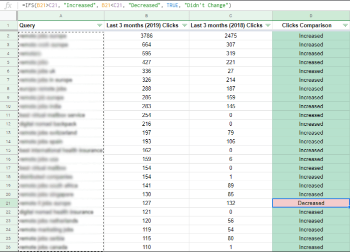
=HYPERLINK("https://www.example.com","Example Website")
This formula creates a clickable link to “https://www.example.com” that displays “Example Website” when the link is selected. Adjust the URL and the displayed text to match your specific needs.
Linking to Other Sheets within the Workbook
Connecting sheets within the same workbook is a fundamental tool for organizing and accessing related data. This allows you to create a cohesive view of your data, whether you are tracking sales figures, project milestones, or other relevant information across multiple tabs.
=HYPERLINK("#'Sheet2'!A1","Sheet 2 Data")
This formula creates a link to cell A1 in Sheet2. The “#’Sheet2′!” portion specifies the target sheet within the workbook. The displayed text is “Sheet 2 Data.” Change “Sheet2” and “A1” to link to any other cell or sheet within the same workbook.
Linking to Specific Cells
Directly linking to specific cells allows for immediate access to data in other parts of the spreadsheet. This is useful when you want to quickly reference information from different sections of your data. This method is useful for creating cross-referencing, improving data flow, and quick lookups.
Ever wished you could quickly reorder rows or resize columns in Google Sheets? There are tons of handy tips and tricks out there! Learning these shortcuts can supercharge your workflow, and honestly, it’s all about maximizing your productivity. A recent development in the content management space has me thinking about Google Sheets organization: TikTok is reportedly testing a standalone content management app, like this one , which will be interesting to see how that impacts creators’ workflows.
Knowing how to efficiently use features like hyperlinks and formulas in Google Sheets will still be a valuable skill, no matter what the future holds.
=HYPERLINK("#'Sheet1'!B3","Cell Data")Mastering Google Sheets is key, especially when you’re juggling reordering rows and resizing columns. Knowing how to link data effectively is super helpful. For example, if you’re tracking Pokémon GO progress during the pandemic, Niantic’s updates and temporary discounts might be tracked in a spreadsheet. Check out the latest on that front in this great article about pokemon go coronavirus niantic updates temporary discounts inside to see how these factors impact in-game strategy.
Once you have that data sorted, you can easily use those linked data points to update your spreadsheets and improve your own analyses on things like best strategies and evolving your Pokémon!
This creates a link to cell B3 in Sheet1, with “Cell Data” as the displayed text. Replace “Sheet1” and “B3” with the relevant sheet name and cell coordinates.
Linking to Ranges of Data
Linking to ranges of data within a sheet is beneficial when you need to present or access a larger block of related information at once. It’s a useful feature for providing context or displaying data in its entirety without having to manually copy and paste.
=HYPERLINK("#'Sheet1'!B3:B10","Data Range")
This formula creates a link to the range B3:B10 in Sheet1, displaying “Data Range” as the link text. Adjust the range to match the data you want to link to.
Comparison of Link Types
| Link Type | Description | Formula Example |
|---|---|---|
| External Website | Links to external websites | =HYPERLINK("https://www.example.com","Example Website") |
| Other Sheet | Links to cells/ranges in other sheets | =HYPERLINK("#'Sheet2'!A1","Sheet 2 Data") |
| Specific Cell | Links to a specific cell within the sheet | =HYPERLINK("#'Sheet1'!B3","Cell Data") |
| Data Range | Links to a range of cells | =HYPERLINK("#'Sheet1'!B3:B10","Data Range") |
Combining Reordering, Resizing, and Links
Mastering the art of data presentation in Google Sheets involves more than just inputting figures. Combining reordering, resizing, and linking elevates your spreadsheet from a simple data repository to a dynamic and interactive tool. This approach empowers users to dissect complex information, extract meaningful insights, and communicate findings with clarity and precision.Effectively using these techniques allows you to transform raw data into compelling visual representations.
Reordering data puts key insights front and center, resizing columns adjusts the presentation for optimal clarity, and linking columns enables the visualization of relationships across different data points. This comprehensive approach fosters a richer understanding of the information contained within the sheet, allowing users to engage with the data on a more profound level.
Scenarios for Enhanced Data Analysis and Presentation
Combining these techniques is particularly beneficial in scenarios where interconnected data needs to be presented and analyzed. For instance, in a sales report, you might reorder sales figures by region, resize columns to accommodate longer region names, and link sales figures to corresponding marketing campaign costs to identify correlations. In a project management sheet, you might reorder tasks by priority, resize columns to display task descriptions fully, and link task completion times to project milestones to track progress.
Example Google Sheet
Consider a sheet tracking website traffic. The sheet contains columns for date, source (e.g., organic search, social media), page views, and unique visitors. By linking the source column to a separate sheet containing marketing campaign details (e.g., campaign name, budget), you can easily understand which marketing efforts drive the most traffic. Reordering the data by date allows for trend analysis over time, while resizing columns to accommodate longer source descriptions improves readability.
A user can instantly grasp the effectiveness of various marketing channels by easily sorting and filtering the data.
Improving User Experience
Employing these techniques significantly enhances the user experience of a Google Sheet. Reordering data by relevance allows users to focus on the most crucial information immediately. Resizing columns ensures that all data points are visible and easily interpretable. Linking data points fosters a deeper understanding by revealing connections between different data sets. Ultimately, this dynamic approach creates a more intuitive and user-friendly environment.
Clarity and Effectiveness of Data Display, Google sheets tips tricks reorder rows resize columns links
Reordering, resizing, and linking significantly contribute to the clarity and effectiveness of data displayed in a Google Sheet. Reordering columns by importance places critical information at the forefront, ensuring it’s the first thing the user sees. Resizing columns to appropriate widths prevents information from being truncated or overlapping, improving readability. Linking columns reveals relationships between data sets, enabling a more comprehensive understanding of the trends and patterns within the data.
Creating a Dynamic and Interactive Google Sheet
This procedure Artikels the steps for constructing a dynamic and interactive Google Sheet using reordering, resizing, and linking features:
- Data Preparation: Ensure your data is organized into separate columns, with appropriate labels. For example, if you have sales figures, include columns for region, product, date, and sales amount. This structured approach is crucial for linking and analyzing data efficiently.
- Linking Data: Use formulas like `=HYPERLINK` to create links between related data points. For instance, create a link from the “Region” column to a separate sheet containing more detailed information on each region.
- Reordering Rows: Sort the data by various criteria using the sort feature in Google Sheets. For instance, sort the sales figures by date or by region.
- Resizing Columns: Adjust column widths to accommodate long text strings or large numerical values, maintaining readability. Use the auto-resize feature or manually adjust the column widths to suit your needs.
- Adding Filters: Add filters to the columns to allow users to view specific subsets of the data based on their needs. This enhanced filtering capability enables a more focused analysis.
- Adding Charts: Create charts based on the linked and reordered data. This visualization can significantly enhance the comprehension of patterns and trends.
Data Validation and Links
Maintaining data integrity in linked Google Sheets is crucial for accurate analysis and reporting. Data validation rules, when applied correctly to linked data, prevent errors and inconsistencies, ensuring that information flows seamlessly between interconnected spreadsheets. This approach not only enhances the reliability of your data but also streamlines your workflow. Linked data often requires careful consideration of validation rules to ensure consistency and prevent mistakes.Data validation rules are powerful tools for maintaining the quality of your linked data in Google Sheets.
By defining specific criteria for acceptable input, you can prevent incorrect or irrelevant data from entering your sheets, ultimately reducing errors and improving the accuracy of your analysis. Implementing these rules in linked data ensures that changes made in one sheet are reflected consistently across all linked sheets.
Data Validation Criteria for Linked Data
Data validation offers a wide range of criteria to ensure linked data conforms to specific standards. These criteria, when appropriately applied, maintain the consistency and integrity of your linked data across different sheets. Ensuring data type and range accuracy is paramount. For example, a column linked to another sheet might require specific numerical values within a certain range.
Validating Data Types
Validating data types is essential for maintaining data integrity in linked spreadsheets. If a linked cell expects a date, a validation rule can prevent the entry of text or numbers. This prevents errors that could affect downstream calculations or analysis.
Validating Data Ranges
Ensuring data falls within a predefined range is equally important. For instance, a linked column representing percentages should be validated to ensure values are between 0 and 100. This approach prevents outliers and ensures the accuracy of linked data.
Automatic Updates with Data Validation
Data validation can be configured to automatically update linked data in other sheets. When a value is entered that violates a validation rule, Google Sheets can provide feedback, preventing erroneous data from propagating to other linked sheets. This ensures consistency and prevents discrepancies across linked spreadsheets.
Example of Data Validation with Links
Imagine a sheet tracking sales figures (Sheet1) linked to a sheet summarizing regional performance (Sheet2). In Sheet1, a column for “Sales Region” uses data validation to restrict entries to predefined regions (e.g., “North”, “South”, “East”, “West”). If a user tries to enter an invalid region in Sheet1, Google Sheets will prevent the entry, ensuring data consistency across both sheets.
Table of Data Validation Rules for Linked Data
| Rule Type | Description | Example |
|---|---|---|
| Data Type | Specifies the acceptable data format (e.g., text, number, date). | Ensuring a column linked to another sheet only accepts dates. |
| Data Range | Limits input to a specific range of values. | Restricting a linked field for “Customer Status” to “Active”, “Inactive”, or “Pending.” |
| Custom Formula | Allows complex validation based on a custom formula. | Validating a linked field ensuring the value is not greater than a value in another cell. |
| List of Values | Restricts input to a predefined list of values. | Validating a linked field with specific product codes. |
Advanced Techniques
Google Sheets offers powerful capabilities beyond basic functions. Advanced techniques allow for more dynamic and adaptable spreadsheets, enabling you to automate tasks, react to changes, and create truly interactive documents. This section delves into custom functions, dynamic resizing, sophisticated linking, and creating adaptable spreadsheets.Mastering these advanced techniques elevates Google Sheets from a simple data management tool to a robust data analysis and manipulation platform.
These methods are crucial for complex projects and situations demanding greater flexibility and control over data presentation and interaction.
Custom Functions for Reordering Rows
Custom functions, written in Apps Script, empower you to reorder rows based on complex criteria. This capability extends beyond simple sorting, allowing for dynamic adjustments to the row order based on calculated values or user input. These functions can be embedded directly into your spreadsheet, providing a powerful tool for manipulating data based on your specific requirements.
- Using Apps Script, you can create a custom function to sort rows based on the value in a specific column. For example, a function could sort by date, amount, or any other relevant column. This allows for dynamic sorting and updates as new data is entered.
- Functions can incorporate more intricate logic. Imagine a function that reorders rows based on a combination of factors, such as date and priority level. This allows for a more nuanced and adaptable sorting strategy.
- Functions can also integrate with other spreadsheet features. For instance, a function could reorder rows based on the results of a calculation or the output of a data validation rule.
Dynamic Column Resizing
Dynamically resizing columns in response to content length or user interaction improves the user experience and optimizes spreadsheet readability. This approach prevents excessive horizontal scrolling and maintains a clear layout, even as data volume changes.
- Implement a script that monitors cell content length within a column. When the content exceeds a predefined threshold, automatically resize the column to accommodate the text.
- Consider a user-interactive method. Allow users to resize columns directly by dragging the column dividers. Implement this functionality using a custom script, ensuring the resizing is consistent with the spreadsheet’s overall design and user interface.
- Dynamic resizing can be triggered by specific events. For example, a column might automatically resize if the data type in a cell changes, or if the number of characters in a cell exceeds a predetermined limit.

Sophisticated Linking Techniques
Advanced linking goes beyond simple formulas. It involves creating complex relationships between multiple sheets and workbooks, enabling data sharing and synchronization.
- Use array formulas for linking data across multiple sheets. This approach allows for efficient data aggregation and manipulation across various parts of a larger spreadsheet.
- Implement Apps Script to manage complex data transfers. This is useful for situations where data needs to be updated across multiple workbooks based on user interactions or external events. For instance, updating a summary sheet with data from several linked individual sheets.
- Utilize IMPORTRANGE to link data from external workbooks or even external data sources, ensuring that changes in external data are reflected instantly in the target sheet. This allows you to work with data that is stored in separate locations.
Dynamic Spreadsheet Structure
Creating a dynamic spreadsheet allows for a structure that adjusts to user input or external data. This enhances the adaptability of your spreadsheets to changing needs.
- Employ conditional formatting to create dynamic sections or tables based on specific criteria. For example, you can display or hide rows based on a particular date range or the status of a project.
- Use Apps Script to dynamically add or remove sheets, columns, or rows based on external data sources. This technique is especially useful when data is received from other systems or applications.
- Implement input validation rules and data entry controls to ensure that data conforms to predefined formats or requirements, thus reducing the chance of errors and streamlining data processing. This is an essential aspect of dynamic spreadsheets.
Concluding Remarks
In conclusion, mastering the art of reordering, resizing, and linking data in Google Sheets unlocks a world of possibilities for enhanced data analysis and presentation. By leveraging these techniques, you can create dynamic and interactive spreadsheets that significantly improve the user experience and efficiency of your workflow. From basic sorting to sophisticated data validation, this guide equips you with the tools to transform your Google Sheets into a powerful analytical tool.